Bikeable
Bikeable is the neural network that can create safety maps for any city, the technology that powers the Route Planner. predicting a safety score for any image, we may then create a safety map feeding thousands of points into the network.

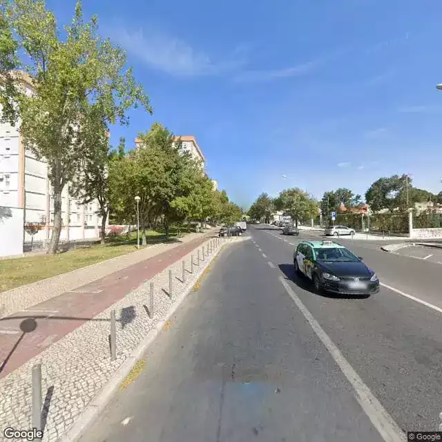

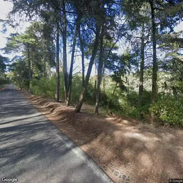
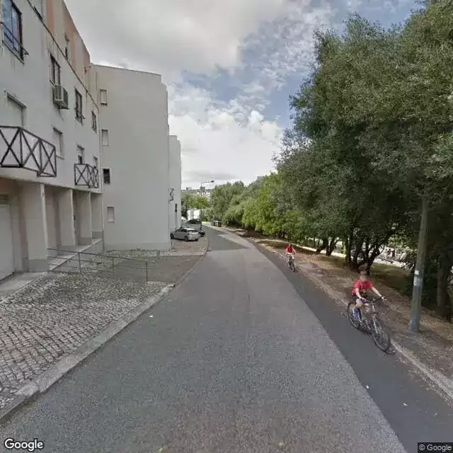
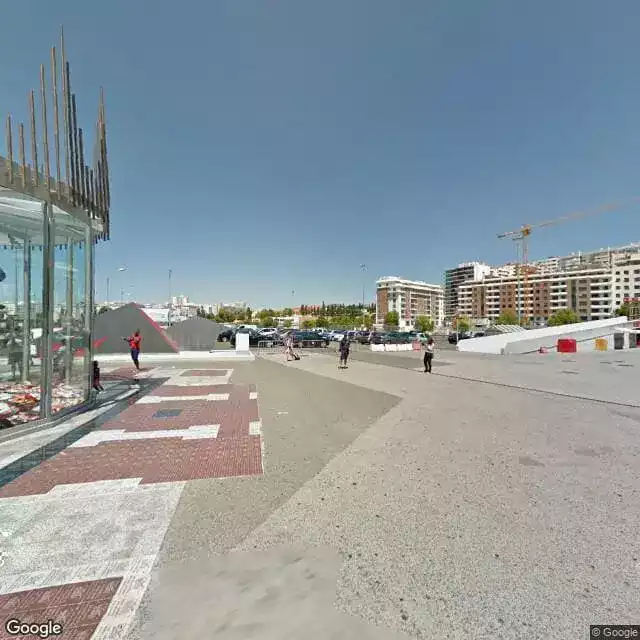


Our model was able to predict with 100% accuracy the safety scores for the top 5 safest and unsafest images from the Bikeable training dataset. Next step consists in validating our tool with unseen data.
Lisbon Safety Map
Bikeable will process 1 000 000 images distributed over 250 000 points from Lisbon. This will allow us to create, for the first time, a cycling safety map for a city with an unprecedented resolution of 20 meters.

For the training, we used 2500 points from the Perception Poll from Lisbon were used. Each point has 4 images, taken from 0-, 90-, 180- and 270-degree orientation, to capture all the information available. Each image had the pixels extracted and counted, correlating them to a particular class, by using the semantic segmentation method developed by NVIDIA (e.g. in image0_270.jpg there were 23423 pixels for the class car). An object detection algorithm, YOLOv5x was used to detect objects present in those images.
A 50% confidence interval was used to discard the bad detections. The results from those 2 methods were combined to serve as an input for the neural network. For the output, the votes from the perception poll were filtered to discard the bad data (e.g. 5 votes in the same second) and a classification algorithm (True Skill) was used to attribute safety scores to images. The multi-layer perceptron neural network was trained using this data, and a 5-fold cross-validation method was used to ensure its accuracy - 70%.
Description
CycleAI's NN - Bikeable - is a MultiLayer Perceptron (MLP) designed to predict the safety score (continuous value from 0 to 10) of an image based on text information. It is trained using Keras Sequential model, which consists of a linear stack of layers. It is composed by an input layer containing 69 nodes, matching the number of features of the dataset, six hidden layers with 69, 128, 64 and 32 units, and an output layer with one neuron, which is typical for regression tasks, where the goal is to predict a continuous value. During the training, the 5-fold cross validation was used, with 30 epochs and a batch size of 3, for all the generated 25 datasets.
Since every image was considered, despite having an object detected or not, the datasets sizes differ due to the sigma/standard deviation restriction (Table 1), removing score records that deviate from the mean by a certain value, eliminating potential outliers.
| Sigma Restrictions | Train Dataset Size | Test Dataset Size | Total |
|---|---|---|---|
| <=4 | 2115 | 235 | 2350 |
| <=5 | 7103 | 790 | 7893 |
| <=6 | 8792 | 977 | 9769 |
| <=7 | 9465 | 1052 | 10517 |
| no restriction | 11952 | 1328 | 13280 |
All hidden layers use the well-known Rectified Linear Unit (ReLU) activation function. The output layer uses a linear activation function, meaning that the output of the neuron is equal to its input.
The model is compiled with Adam optimizer, a widely used optimizer that adapts the learning rate during training. This is advantageous because it combines the benefits of two other extensions of stochastic gradient descent: AdaGrad, which works well with sparse gradients, and RMSProp, which works well in online and non-stationary settings.
The model uses Mean Squared Error (MSE) as the loss function, a popular choice for regression problems because it penalizes larger errors more than smaller ones, leading to a more accurate model. It also tracks Mean Absolute Percentage Error (MAPE) during training as a metri
Due to the overfitting observed, a larger dataset was selected for further experiments. Taking into consideration the insights gained from previous experiments, the dataset with sigma less than or equal to 5 and an OD confidence threshold of 70% demonstrated the highest training accuracy among the larger datasets. After performing the evaluation using the test set, the original model with this dataset did not overfitting, therefore, the focus shifted towards improving the accuracy of the model. After 5-fold cross validating multiple models with different hyperparameters, such as number of layers, batch sizes and regularization parameters, the averaged accuracy was increased to 82,19% (Table 2). The model was run for 60 epochs with a batch size of 32.
| Averaged Metrics | Standard Deviation | |
|---|---|---|
| Average MSE | 1,08 | +/- 0,25 |
| Average MAPE | 17,81% | +/- 2,44 |
| Average RMSE | 1,02 | +/- 0,12 |
| Average MAE | 0,81 | +/- 0,10 |
| Average R Squared | 0,37 | +/- 0,13 |
| Average Model Accuracy | 82,19% | +/- 2,44 |
In addition to increasing the number of epochs and utilizing a batch size of 32, other modifications were made to the model. Specifically, a hidden layer with 64 units was incorporated, and four dropout layers were added after every four initial hidden layers. The model's structure can be seen in Table 3.
| Layer | Neurons | Activation Function |
|---|---|---|
| Input Layer | 69 | |
| Hidden Layer 1 | 69 | Relu |
| Dropout 0.1 | ||
| Hidden Layer 2 | 128 | Relu |
| Dropout 0.1 | ||
| Hidden Layer 3 | 64 | Relu |
| Dropout 0.1 | ||
| Hidden Layer 4 | 64 | Relu |
| Dropout 0.1 | ||
| Hidden Layer 5 | 32 | Relu |
| Hidden Layer 6 | 16 | Relu |
| Hidden Layer 7 | 16 | Relu |
| Output Layer 7 | 1 | Linear |
The evaluation on the test set yielded a 79,09% model accuracy (MAPE=20,91%).